v1.0 - Initial draft

What I’ll talk about #
I started Didact AI in 2019, out of a firm belief that stock picking engines built on top of machine learning models could consistently beat the market, gaining and retaining profits.
I worked on this idea full-time for 2 years, from 2019 to 2021, building a stock picking engine that actually generated outstanding returns, steadily beating the S&P 500 for over a year on a weekly basis.
Once the engine was ready, I started sending out a weekly newsletter to a handful of subscribers from June 2021 to July 2022, with stock picks for the next week, in conjunction with a simple risk management play, and demonstrated the engine’s prowess through multiple market crises, with steady out-of-sample outperformance available to the newsletter subscribers. In the meantime, I added an engineering co-founder and a marketing maven to assist with the rollout.
And then, for a variety of reasons (mostly to do with the perceived lack of PMF), we pulled the plug and shut down the newsletter service.
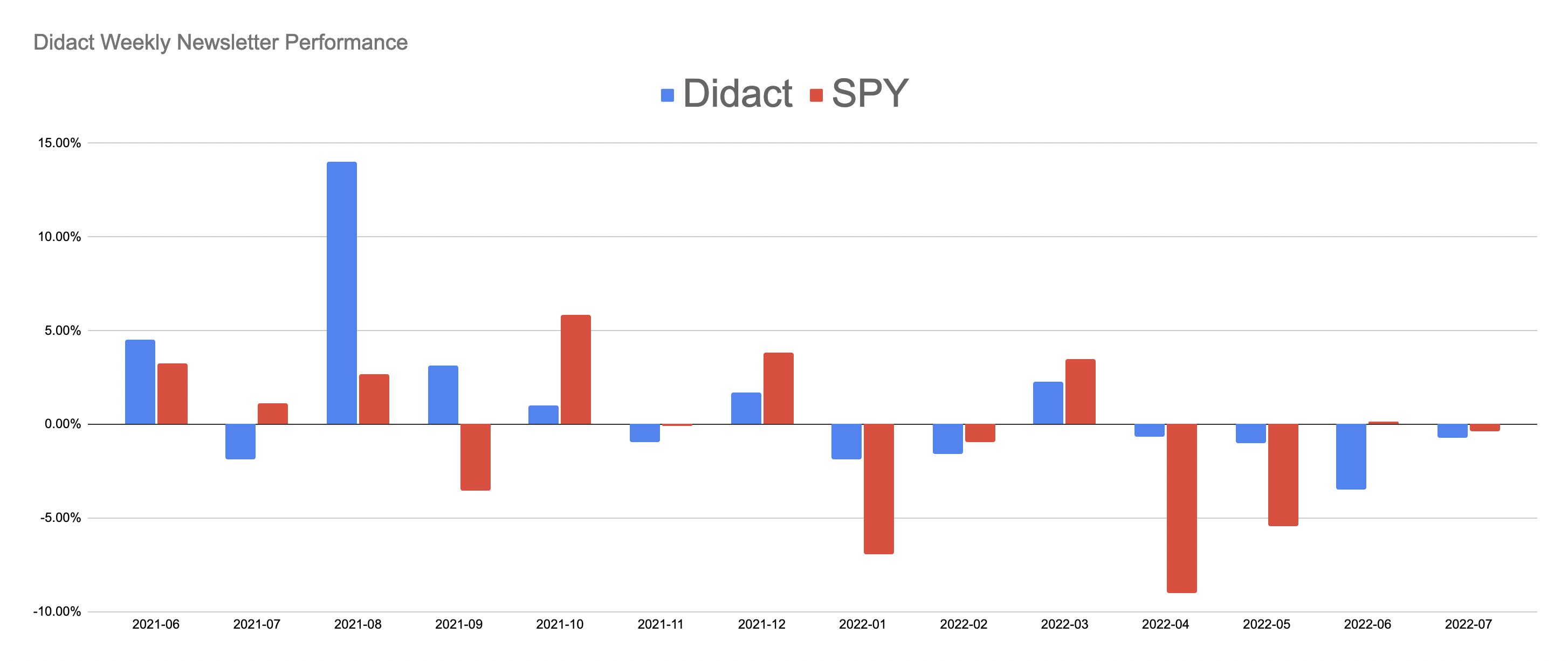
It was quite amazing while it lasted though. Here are some summary performance metrics from the engine’s real-world predictions (May 31, 2021 - July 8, 2022):
| Performance Metrics | SPY | Didact |
|---|---|---|
| Avg Rtn (Wkly) | -0.09% | 0.25% |
| Std Dev (Wkly) | 2.55% | 2.19% |
| Downside Dev (Wkly) | 1.22% | 0.39% |
| Avg Rtn: SPY is +ve (Wkly) | 1.84% | 0.85% |
| Avg Rtn: SPY is -ve (Wkly) | -2.03% | -0.31% |
| Sharpe Ratio (Ann) | -0.27 | 0.83 |
| Sortino Ratio (Ann) | -0.56 | 4.64 |
| Corr w/ SPY (Wkly) | - | 0.18 |
| Total Return (Jun 2021-Jul 2022) | -7.1% | 14.2% |
| Return (Jun-Dec 2021) | 13.6% | 22.7% |
| Return (Jan-Jul 8 2022) | -18.2% | -6.9% |
If this intrigues you, read further.
The strength of Didact’s predictive performance lies mostly in its engineered features and modeling approach, but the architecture and technology used played a significant role as well.
In this essay, I will focus on the latter, briefly digressing at times to the principles and assumptions behind the system, with detailed walkthroughs of the separate data ingestion pipeline, feature engineering pipeline, and modeling subsystems, essentially covering the data engineering, modeling, ML engineering, and ML Ops tasks that were required to pull this system together. Through this essay, I hope to convey an idea of how productionized ML systems work in a real-world setting.
I have tried to write this essay in as self-contained and comprehensive a manner as possible (though it does require a basic knowledge of how machine learning works), while not completely giving away my trade secrets (ha!). I will continue editing this over the next few days (I have already identified a few disjointed sections), but in the meantime I hope you enjoy reading it as much as I did writing it.
Markets: Patterns, Regimes, Regime Shifts, and Sentiment #
I want to quickly cover some of my assumptions / structural priors on how I think markets work. Hopefully this level-setting will make reading the rest of the essay more palatable.
We will start with market patterns, which are chunks of similar price-volume actions repeated across time. Whether expressed visually as a chart pattern or a more complex multi-market time-series artifact, patterns are fascinating entities; structured on the interplay between price, sentiment, and market regime (in the broadest sense possible), they are ephemeral in nature, appearing for a few days or weeks and then rapidly morphing into something new. The traditional idea behind chart patterns (and technical analysis) is that when certain patterns appear, it is easy to predict the trajectory of the underlying stock going forward.
However, as patterns evolve through time, the payoffs for anticipating and trading their trajectories change as well. A pattern that might have been profitable on the long side might see its edge erode and become nonpredictive as other speculators (whether humans or machines) tack on, and yet reappear after months or years with its predictive character back. The reason why this happens is most likely that humans behave in certain predictable ways in certain situations (eg “markets are collapsing, move to Treasuries”), and this manifests in market regime behavior with divergent trajectories for expected returns in equities and other asset classes. In other words, it is important to contextualize market patterns in terms of the “regimes” in which they appear.
Let us now dig deeper into market regimes. These can be roughly thought of as the “context” in which individual assets operate. For example, an asset whose cash flows depend on energy commodities will be intimately tied to WTI crude oil futures prices and corresponding geopolitical sentiment. The latter is part of what makes up a market regime. Think of it as a mathematical summary of where markets and economies are currently situated in relation to each other and in relation to their own histories. Using this operational definition of a market regime allows us to model both asset dynamics as well as market dynamics together.
One thing to keep in mind is that, depending upon the level of analysis required, market regimes may be as fine-grained or coarse-grained as required. For instance, a basic market regime model may take as input equity index prices and determine whether one is in a bull market or a bear market (i.e. 2 regimes). At other times, more sophisticated market regime models (such as the one used in the Didact engine) may best be described as exhibiting hundreds of regimes, each with its own unique dynamics and forward return biases.
So what are regime shifts? Think of these as sudden switches from one market regime to another, mostly due to exogenous circumstances, which are reflected in asset class returns and individual asset repricing. This repricing will happen as market participants reallocate capital, selling out of one class and buying into others.
Individual regimes may be long-lived or short-lived, but typically last for 21-35 days (mean/median) as per my analysis, while regime shifts may take place very quickly (overnight or during the market open or closing auction), or may slowly grind their way through the better part of a day.
Finally, let’s talk about market sentiment. Think of this as aggregated bullish or bearish behavior exhibited across assets (“I’m bullish on Apple/Tesla”) or asset classes (“Tech is where most money will be made next decade”). Market sentiment, reflecting aggregate participant behavior, is best captured in the form of relative trading volumes weighted by periodic returns, e.g. high negative (positive) returns in conjunction with high volumes are a strong signal of prevailing negative (positive) sentiment about the underlying asset. Note that the size of the returns and volumes should ideally be mapped against the asset’s (or equity’s) cohort (e.g. others in the same sector, industry, or index).
Market sentiment exhibits an interesting phenomenon during regime shifts, during which certain assets move in lockstep over smaller timeframes, adding credence to a famous market truism that during market crises, all correlations tend to 1.
To recap:
- market patterns (e.g. a stock trading near the 20-day low, 5 days after a terrible earnings release)
- may exhibit predictable forward trajectories, when analyzed in conjunction with
- market regimes (e.g. US indices trading sideways last 2 weeks, with volatility indices at monthly lows) and
- sentiment (e.g. surge in S&P 500 daily volumes, with a similar surge in S&P 500 put volume for expiry in 2 weeks).
These concepts, stitched together, power the Didact engine’s predictions.
Engine architecture: A 50k ft view #
Like most machine learning systems, the Didact engine is best viewed as a pipeline that processes raw financial market data at one end and spits out the latest stock picks at the other end. Of course, deploying the Didact engine into a production context faces the same issues as any other ML-powered system. Both tackle the same quandaries - how to measure performance on a real-time basis, how to incorporate dynamic feedback signals, how to identify signals that indicate the underlying system is “overheating” and so on. The components are fairly similar as well: a battery of data cleansing pipelines that run on data that’s streaming in from a variety of sources, followed by feature engineering and filtering processes that in turn feed into full-blown action-oriented modules (execution systems in the case of trading, recommendations and/or insights in the case of ML). The case for a control panel is immediately apparent, as is the need to insert and maintain long-running monitoring processes that keep tabs on system health.
With that in mind, here’s a 50,000 ft view of the Didact architecture:
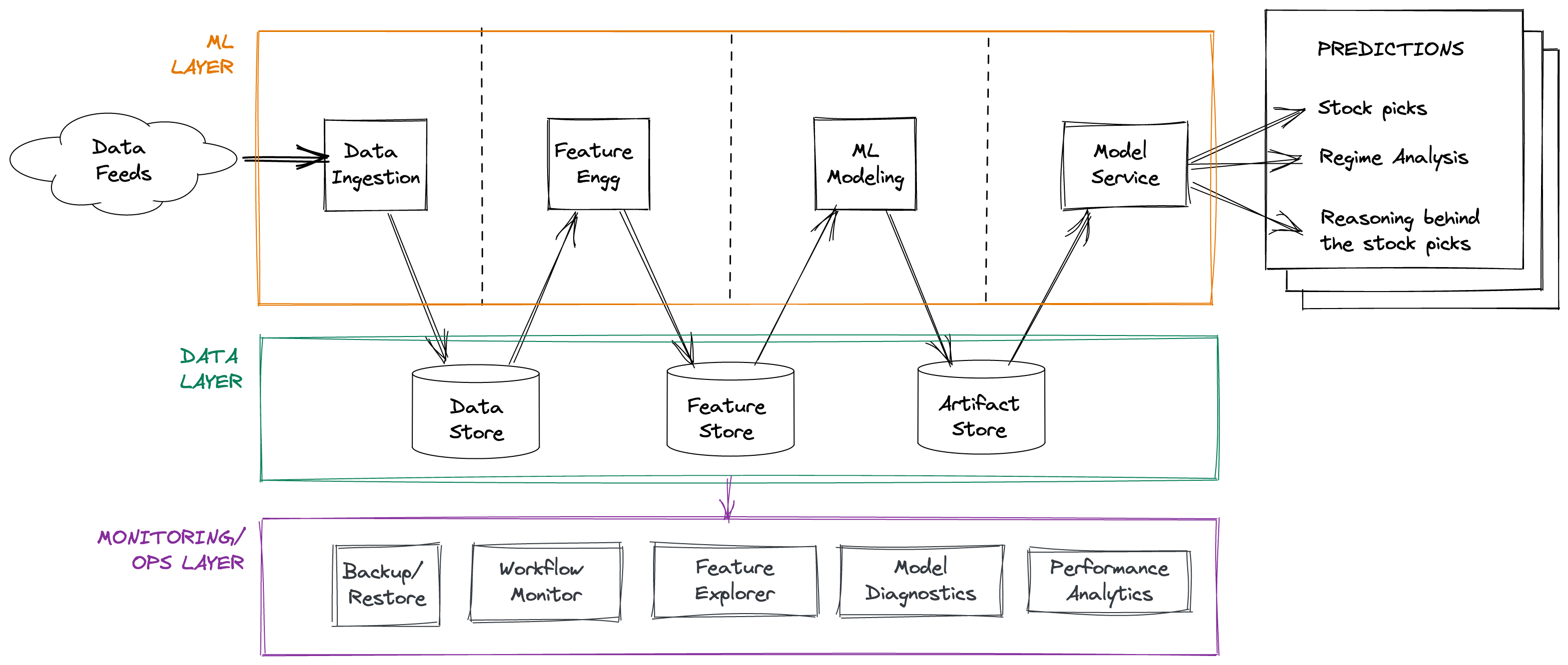
Of course, this obscures a lot of details. We will dig into each of the components in the following sections. Having said that, here are some general points to keep in mind.
Design focus #
My main aim with this architecture was to make it easy for the Didact AI ML team (i.e. me) to be able to perform rapid experimentation with feature engineering. From my time in the trenches both as an ML researcher and as a systematic quant trader, an insight I have always kept in mind is that feature engineering is almost always the key difference between success and failure; once you have strong features for your problem domain, to butcher Wolpert’s “No Free Lunch” theorem, the choice of ML model is no longer a critical step.
My secondary aim was a relentless focus on execution speed. The analytics requirements are heavy: on a daily basis, the pipeline must process text and time-series data for over 4000 US stocks, ETFs and macroeconomic series, generating 1000+ individual features for each stock that take into account the web of complex relationships across sectors, industries, indices and fund ownership-imposed bundling.
As another example, occasionally (1x a quarter per listed stock), I have to fetch and process earnings call transcripts and SEC EDGAR filings (10-Qs) and use deep learning-based language models to identify changes in how corporate leaders think of their own company and the environment in general. This is a compute-intensive process, one that I tackle by offloading web scraping and model-based feature extraction to a weekly run; the reason being that since earnings releases tend to cluster together on the calendar, it makes sense to run a higher-end GPU-equipped EC2 instance periodically and batch-process a bunch of filings together, making for large savings on compute costs.
Due to the reasons mentioned above, I expended a lot of effort reducing the raw data->insight timeline, and I successfully managed to bring it down from roughly 2.5 hours when I started, to ~35 minutes by the time we were ready to go live, finally ending with an ~14 minute pipeline run.
Tech stack #
The modules in the ML layer are written almost exclusively in Python (it being the preferred language for machine learning), though some parts of the pipeline were re-written in SQL (mentioned below), and some bottlenecks were tackled by swapping out Pandas with higher-performance alternatives. I will talk more about this in the Tackling Performance Bottlenecks section. These layer modules are executed sequentially, with corresponding preconditions (input validations) and postconditions (quality checks).
The data layer is composed of three separate stores, because of the differing access patterns that they support:
-
The data store: I initially used Postgres as a data store to capture data post-ingestion; there were significant speed issues due to my heavy use of table columns as features. I eventually moved the data store over to DuckDB, which is a column-oriented embedded DB with excellent performance characteristics, that plays quite well with Apache Arrow and Parquet.
-
The feature store: I used Redis as a feature store (initially as the only store), persisting to disk. On top of core Redis, I developed a feature access layer that let me perform fine-grained feature engineering while also doing aggregations (more about this here). I have now augmented Redis with DuckDB, again because of the wonderful performance characteristics of the latter that complement Redis’ capabilities. This addition has enabled me to push a large number of basic feature engineering routines down to SQL scripts (mimicking relevant Pandas semantics through a liberal use of WINDOW functions) for rapid columnar processing.
-
The artifact store: This is on-disk local storage that gets backed up to AWS S3 every day. Only the last 60 days’ worth of artifacts are retained locally on disk. Artifacts include serialized models, model forecasts, market regime metrics and forecasts, and training data snapshots.
The ML Ops / monitoring layer is composed of separate modules that together serve to track the data exhausts of the ML layer. These modules are written in Python and are invoked as command-line scripts that generate reports, with the exception of Feature Explorer, which I use extensively to experiment with feature engineering ideas.
Python environment setup #
The engine is built on a Python 3.8 Conda environment. The most relevant packages in the environment for this discussion are:
- Data engineering: duckdb, numpy, pandas, pyarrow, boto, redislite
- ML Modeling: jupyter, pandas, numpy, polars, joblib, bottleneck, pytorch, tsfresh, transformers (from huggingface), xgboost, scikit-learn, scipy
- ML Ops: dash (from plotly), fastapi
Beyond this, I leverage the Python standard library as far as possible, using multiprocessing judiciously to use all the cores at my disposal for compute-intensive tasks that are not amenable to GPU-style processing. I would have liked to use NVidia’s RAPIDS set of libraries to speed things up further, but, and this is not surprising, cloud GPUs are expensive.
Execution platform #
We used AWS for our infrastructure needs. The pipeline was executed on a r5a.2xlarge instance (8 vCPUs, 64 GB RAM) optimized for intensive in-memory compute, with an attached EBS volume. We self-hosted Redis + Postgres on our EC2 instance. Data+artifact backups were stored in private, locked down S3 buckets.
Pipeline scheduling #
The engine is executed 2 hours after the end of every trading day. This gap is maintained to allow the external data providers to refresh their datafeeds (e.g. cleaning and processing the latest day’s action/festivities). Quality checks on the incoming data are performed and if necessary the external providers are re-polled until all checks pass.
When the engine was in production last year, we scheduled pipeline runs using cron jobs to execute shell scripts calling individual Python modules. Notice, though, that the pipeline essentially describes a DAG of tasks that can be executed in sequence (sometimes in parallel). I am now in the process of rewriting the pipeline to take advantage of Apache Airflow as a DAG orchestrator.
Though the engine is run every day, stock picks are extracted only from Friday’s run (or from that of the last trading day previous week). This is done primarily to reduce cognitive burden; trading in and out weekly is tough enough as it is, but changing portfolios on a daily basis might be an insurmountable burden for individual investors.
Interlude: Complexity in financial data #
Financial data is multi-modal (spanning text, time series, and implicit network graphs) and incredibly complex.
As an example of data complexity, the options datafeed contains bids/asks, volumes, open interest, implied volatility, etc. for all the options contracts currently being traded for a given symbol at a given date, grouped across time (25 days to expiry, 46 days to expiry, etc.), strike price (350 series, 450 series, etc.) and type (call/put). As time goes by, some of these options will expire and drop out of the datafeed, only to be replaced with new contracts.
Meanwhile, the underlying symbol may undergo corporate changes such as a name change, ticker change, stock split, reverse split, spinoff a subsidiary, merge with another company, or acquire something else, and so on. I built tooling around my external data providers’ reference datasets in order to track and trace these changes, so that the downstream feature engineering pipeline may continue to assume a single corporate entity existing through all of these evolutions. (Note that such corporate actions are by themselves rich sources of informative features; I mine them separately.)
For extraordinary situations such as Google’s famous reorganization into Alphabet and its subsidiaries in 2015, it is perfectly okay to create one-off scripts that synchronize pre-event and post-event data.
Another important type of event to track is the reconstitution of indices, where new companies are added to an index, and some old companies drop out. For major indices such as the S&P 500, or the Russell 1/2/3000 series, reconstitution dates are announced in advance, and additions/removals are announced well before that. Since passive index managers are forced to buy and sell in bulk to maintain their tight tracking of the underlying index, these reconstitutions trigger massive capital flows in and out of specific stocks, sectors and industries on a periodic basis. And yet, even though the dates are known in advance, there is still marginal alpha to be obtained by capturing these events as informative features (most recently during the Russell index reconstitution in June 2022).
Beyond this, it is important to track dates on the calendar for important events such as Federal Reserve FOMC meetings, state and federal holidays, options expiry days, futures expiry days, triple witching and quadruple witching days, macroeconomic releases (monthly nonfarm payrolls and associated unemployment data), and so on.
Finally, when processing earnings call transcripts and EDGAR filings, both of which are text-based and amenable to analysis by SOTA language models, one can infer crucial insights about corporate officers’ uncertainty around the future prospects of their company, simply by capturing changes (and variance) in topics, word frequencies, and sentiment. These features are especially useful in the aggregate e.g. if most earnings calls in a particular sector/industry are more upbeat “than usual” (how to define this is left as an exercise to the motivated reader), it may indicate better-than-average market performance for that sector or industry.
The data ingestion pipeline #
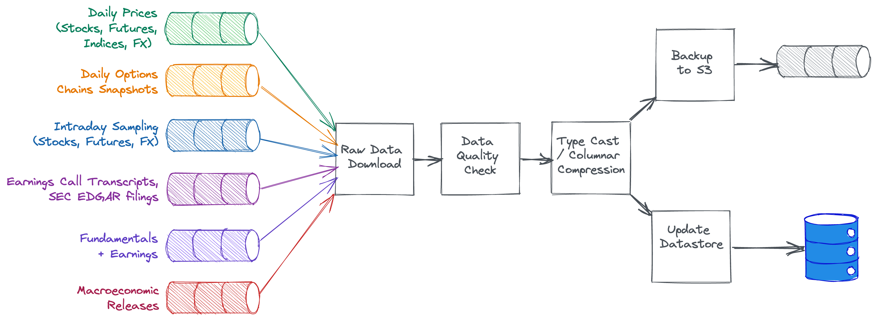
While the amount of raw data ingested and processed by Didact on a daily basis is small (~0.5 GB per day), it is quite complex, distributed across multiple input feeds, with several cross-cutting relationships that need to be kept in mind in order to avoid downstream processing errors.
This is how the ingestion pipeline looks:
Data taxonomy #
As you can see above, the Didact engine processes a wide variety of data. Here’s how it all breaks down:
| Data feed | Frequency | Asset Class Coverage | Type |
|---|---|---|---|
| Price/Volume Data | Daily | Equities, Futures, Indices, FX | Snapshots |
| Options Chains | Daily | Equities, Indices | Snapshots |
| Intraday | 1 minute | Equities, Futures, FX | Timeseries |
| Earnings Call Transcripts | Quarterly | Equities | Unstructured text |
| EDGAR filings | Quarterly | Equities | Structured text |
| Fundamentals + Earnings | Quarterly | Equities | Snapshots |
| Macroeconomic Releases | Varies (Weekly, Monthly) | N/A | Snapshots |
Some quick notes:
- Snapshots are when the data provider pushes out summary data points (usually for a day). These need to be stitched together by the data ingestion pipeline into a coherent multidimensional time series.
- FX refers to currency spot markets. Our data providers source this by blending together quotes and prices from a range of dealers.
- Indices refer to equity indices, but also non-conventional indices such as the VIX.
- Macroecoomic Releases include weekly (e.g. initial jobless claims) and monthly releases (nonfarm payrolls, GDP numbers). These are snapshots that need to be stitched together by the data ingestion pipeline into a time series.
Data quality #
The pipeline run begins by grabbing the latest day’s data for all US stocks and reading them into PandasArrow DataFrames. Some basic quality checks are then performed (e.g. are there any stocks that don’t have data today, that did have data yesterday? did the stock get delisted or was trading stopped? if not, we poll the data providers again, repeating the process until all “active listed” stocks have had their data captured).
Sometimes, rarely, data providers publish bad prints - e.g. a stock whose recent price has been around $500 gets a closing price of $2. Quality checks are put in place to capture such cases, by looking at unlikely implied returns (e.g. price changes that are hundreds of standard deviations away from the average price change) and comparing lists of such stocks with those that have gone through some form of corporate action recently (e.g. splits, reverse splits, mergers, acquisitions, and so on) that may affect the price dramatically. If the former stock does not appear in the latter list, it is likely to be a bad print, and is worth re-fetching from the provider after a certain amount of time (this is set at default to another 2 hours).
Quality checks are currently written in pure Python - using Great Expectations as a framework to compose and maintain these data quality tests is on the roadmap for the engine.
Columnar Compression / Basic Transforms #
Almost all of the commercial data feeds processed by Didact exhibit varying degrees of denormalization in their data. This redundancy is super-expensive to store and to process downstream, which is why after the battery of quality tests are passed, the ingestion pipeline performs some normalization steps, applying column type casting (e.g. marking symbol names as Categoricals) and dropping columns, and maps timestamps to a proprietary pair of (date, time) uint16s, further reducing space requirements (especially important when handling options chain data).
The data is now ready to be pushed from DataFrames into DuckDB.
Backups #
One of the ML Ops scripts is responsible for picking up the new updates to the data store, saving them to Parquet files and pushing them to AWS S3. The advantage of this method is that, in the unlikely case of a Restore, the backed up Parquet files don’t need to go through a compression/basic transform stage again, and fulfil data quality mandates.
Interlude: How I think about ML in markets #
On the surface, it seems quite easy to cast financial market forecasting in a machine learning mold. Let’s peel this onion a little bit.
-
supervised learning: casting the forecasting problem might be thought of as regression (e.g. predict tomorrow’s return for MSFT, minimizing RMSE losses), or it could be thought of as classification (e.g. predict whether MSFT will beat SPY over the next 5 days, minimizing binary cross entropy losses).
-
unsupervised learning: The forecasting problem may also be reduced to an unsupervised learning problem of discerning market regimes, modeled as distinct clusters of market data, with associated forward trajectories conditioned on a ticker, index, or asset class.
-
self-supervised learning: This form of casting is also prevalent in classical autoregressive time series analysis (e.g. ARIMA models), but one could also formulate this as masking some parts of the feature vector and using other parts to predict the masked data.
-
learning to rank: One could think of forecasting as a way to rank each stock relative to each other, on the basis of expected forward returns; this classic formulation comes to us from the field of information retrieval, but is well-suited for a stock picking task.
-
recommender system: Borrowing concepts from recommender system theory, one may choose to model stocks as items and market regimes as users, the idea being that a recommendation would entail matching the most appropriate stocks for a given market regime, using some well-established algorithms such as collaborative filtering.
-
reinforcement learning: This is a fairly popular metaphor in financial markets; the idea being that one can think of stock picking as materialized trading agents that seek to maximize their rewards in the form of total (or average) return on investment over a large time period by taking actions such as buying or selling some stocks.
Ideally we want to be able to pick the best ideas from each sub-field of machine learning and blend them together into one high-performing robust system.
Feature Engineering pipeline #
This is how a feature vector (representing a single stock at the End-Of-Day for a given date) looks like:
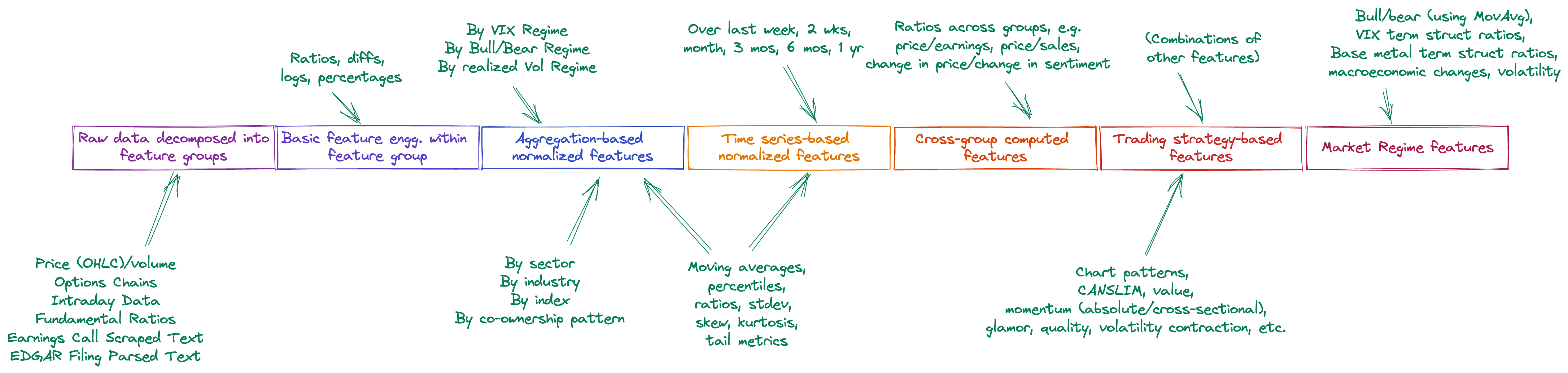
As can be seen above, the feature vector is composed of bundles of features, each bundle using a different methodology to arrive at its feature values:
- It starts with raw features extracted from feature groups, which correspond to a type of processed data (e.g. price/volumes, options chains, sentiment extracted from the text data etc.).
- Next, some basic feature engineering is performed within each group, e.g. from price/volume data, one may derive (Close-Low)/(High-Low), a measure of where the closing price for the stock was in relation to the overall range established for that day. There are scores of these features computed at this stage.
- Now, each of the previous engineered features is contextualized and normalized by comparing the stock’s data against that of its peers, belonging to the same sector, industry, index, or within an exhibited co-ownership pattern (i.e. the same large hedge fund owns this stock and others). Percentiles are computed at this stage among other things. Note that, since stocks may change sectors, industries or indices, it is critical to maintain as-of-date reference data about such events.
- The stock’s data is also contextualized on its prior history, e.g. its closing price is compared against that of the closing price in the last 1 year; similar to the previous stage, percentiles and ratios are computed, along with statistical measures such as standard deviation, skew, and kurtosis. By definition, these are computed on a rolling window basis.
- Cross-group features are now computed; this is where features such as price-to-sales, price delta over sentiment delta, etc. are computed, traversing feature group boundaries. These features enhance the accuracy of the trained model.
- Trading strategy-based features encapsulate the idea that some strategies may be profitable (i.e. be directionally correct) during certain market regimes. Accordingly, the engine runs a bunch of trading strategies, covering technical analysis, momentum/trend following, value, quality, low volatility, skew, glamor, etc. and captures the predictions as features.
- Finally, market regime-based features are also included, inserting information about the current state of the market on that day. Information is captured about the VIX term structure, the S&P 500’s current position w.r.t. its 200-day moving average, the shape of the US yield curve, the realized trajectories of macroeconomic releases such as unemployment, housing starts, housing sales, consumer confidence, and so on.
I would be remiss if I didn’t mention this: the piece-de-resistance of the feature vector design is the addition of, as a feature, the accuracy gap between the latest predictions and the actual realized values, expressed as percentages. This feedback loop helps the training model detect regime shifts quicker.
Event time vs chronological time #
One fascinating source of ideas about features comes from thinking about time differently. Due to a historical quirk, we are used to receiving financial data that’s aggregated at a per-minute, per-hour, per-day, etc. level, basically using chronological time (“clock time”) to measure changes in the underlying entity. And this seems fairly normal.
However, if we were to switch our reference and look at the data from an “event time” perspective, we would be measuring the passage of “time” in the form of event counts instead, aggregating data on a per-100 trades, per-1000 trades, etc. basis, thus giving rise to the concept of “volume bars”.
In many ways, this is similar to moving from the time domain to the frequency domain in signals theory, and the payoff is the ability to design new ML features that capture inverted time-related information. Though we don’t have access to data at trade-level granularity, we can make a reasonable approximation of event time-based features by “inverting” 1-minute data. Let’s leave it at that.
ML Modeling subsystem #
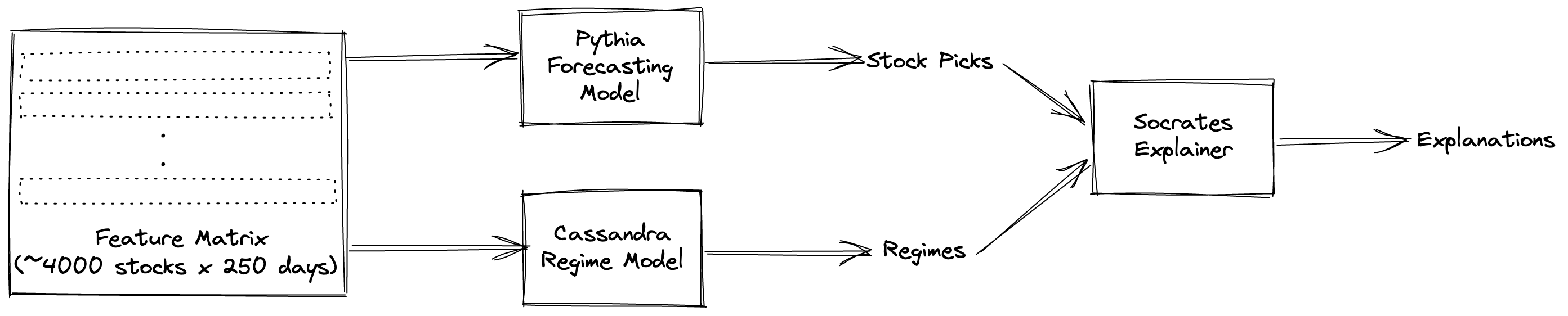
Feature matrix and modeling approach #
The forecasting model is trained on a feature matrix consisting of ~4000 stocks, whose features have been computed for the last 250 days that we have forward data for. This training dataset contains about ~1 M data points, which is sufficient to train a fairly complex gradient boosted tree model.
Why gradient boosting? Random forests are not a great fit for this problem, since it is quite likely that the current market regime may have never been seen before, and the dataset may thus be imbalanced; GBDTs are generally better at handling imbalanced data.
Why not deep learning? For starters, the size of the dataset is too small. It would also necessitate changing the entire modeling approach. I do have some ideas on this front involving transformer-based architectures; hmu if you want to chat about it.
Pythia: Forecasting Model #
In the engine, I use xgboost to train a forecasting model; the target is to pick those stocks that have a >75% probability of generating forward Sortino ratios>2.0 times that of the S&P 500 (in the form of SPY). If the engine scores more than 20 such stocks, it picks the top 20, sorted in descending order of probability.
This forecasting model is retrained every day! Yes, even though it is only used once a week, I like to keep track of regime shifts as and when they occur, and many times the latter may happen in the middle of a week.
Cassandra: Regime Model #
The regime model tracks the current market regime, and computes forward trajectory projections for the S&P 500, Nasdaq, and Russell 2000 indices. Internally, the engine also maintains forecasts of which regime the markets will shift to next; this is important since the regime model’s forecasts are critical to having a strongly performing forecasting model.
The regime model focuses on a subset of columns of the feature matrix that have to do with index-level aggregated information.
Socrates: Model explanations #
It is important to not only get stock picks from the engine, but also a sense of why these particular stocks were picked. The Socrates module provides these explanations, by constructing a narrative for each prediction. Behind the scenes, I use shap to generate these explanations from the model, and then process them to make them human-comprehensible.
The next version of Socrates will incorporate natural language generation so that the engine can provide a succinct sentence or two explaining its reasoning behind the stock picks.
ML Ops: Forecasting and Monitoring #
You can think of this layer as the control plane for the overall engine. Modules in this layer are mostly invoked manually, with the exception of the automated backup script.
The primary objective of this layer is to monitor the main ML layer (the pipeline) for outright errors, subtle bugs, and potential catastrophic drops in profitability. Though the latter is less likely due to the way the engine is designed to account for rapid regime shifts, it is still something that needs to be tracked.
The secondary objective of this layer is to take a virtual magnifying glass to individual features - once I define a feature, I like to study it to observe potential drifts, patterns, correlations, and so on. These in turn may lead me (and occasionally have) to figuring out new features that may capture market aspects that I haven’t yet thrown into the mix.
Backup/Restore #
The backup module is straightforward: it makes backup copies of the following to private AWS S3 buckets:
- “raw” data out of the data store, stored as Parquet files
- serialized model binaries
- model predictions, timestamped
- market regime forecasts, timestamped
- feature matrices, timestamped
- training data snapshots, timestamped
Nothing gets deleted from the S3 buckets.
The restore module does the reverse, not unlike a simplified rsync; copying over files from corresponding S3 buckets back to local storage, while maintaining a time window restriction (e.g. last 60 days’ worth of data).
Workflow Monitoring #
The workflow monitoring module is a script that analyzes logs from the main ML pipeline and sends me a SUCCESS Report or a FAILURE Report (with stage-based diagnosis of the error) via email.
I plan on upgrading this to a browser-based admin panel.
Feature Explorer #
The idea behind this is to have a mechanism for me to explore already-constructed features and let my imagination run wild in terms of thinking up new features. Once I think of a new feature, I can rapidly test it in a Jupyter notebook and, if it’s any good, I’ll add it to the appropriate stage of the feature engineering pipeline.
Here’s a really early version of this module (back when Didact was called GrowthStocker :grimacing: and only processed data from 2 feature groups: price/volume and fundamentals) - I built the UI using Plotly Dash with Bootstrap components:
Model Diagnostics #
The model diagnostics module traces model predictions, compares them against realized returns, and tracks how the delta between the two evolves through time (both on a backtested as well as walkforward basis). Though individual models may change, dramatic spikes in accuracy gapping may indicate something has fundamentally changed in the markets that needs to be incorporated into the Didact engine.
Performance Analytics #
This module is the flip-side of the diagnostics module, tracking model performance as measured in returns of a hypothetical portfolio, compared against SPY. It keeps track of standard trading metrics such as Sortino ratios, Sharpe ratios, volatility, downside risk, win/loss ratios, profit factors, and so on.
Tackling performance bottlenecks #
These are the changes to a standard machine learning workflow that I incorporated, that helped in speeding up the execution of the pipeline:
- Replacing Postgres with DuckDB. The latter’s in-memory columnar processing tooling proved immensely useful; the columnar orientation was especially helpful since it’s critical to do bulk vectorized computations during the ingestion phase.
- Replacing pandas with PyArrow and DuckDB in the ingestion pipeline. I used PyArrow to read in the snapshot data, clean and recast columns quickly using PyArrow tooling, and then perform zero-copy loads into DuckDB.
- Replacing numpy with bottleneck in the feature engineering pipeline. Bottleneck is a library of fast Numpy functions in C; substituting these functions in place of their Numpy counterparts saved a ton of CPU cycles.
- Replacing pandas with polars in the feature engineering pipeline. Polars is a supercharged DataFrame library written in Rust that is closely integrated with the Apache Arrow ecosystem. Using Polars instead of Pandas helped me pile on the speedups, though some care was necessary since the functions don’t map one-to-one.
- Redesigning the ingestion and feature engineering pipelines to take advantage of multiprocessing. Vectorization may only take you so far; using all the cores on your EC2 instance is a much better use of resources.
Coda: Why I shut down Didact #
In a bull market, everyone’s a genius.
By the time I launched the newsletter (June 2021), the great COVID bull run (fueled by stimulus checks, zero-fee brokerages, crypto bull runs, and the lack of things to do outside) was beginning to peter out.
Now, it’s far easier to make money in a bull market, since you can throw a dart and hit a winning stock; it’s tough to stand out on the basis of your performance alone, though, since the latter will invariably fall short against the self-proclaimed genius who bought GME at $10 and sold at $350.
On the flip side, it’s tough to make money in an unstable and rapidly changing market, but easier to stand out, as your performance will show really well against participants who have made double-digit losses on their speculative plays. Unfortunately, if your target market is the same group of participants, you will be fighting an uphill battle against the mother of all behavioral biases, loss aversion; this bias will manifest itself in customers pushing back against allocating capital to your systematic stock picking engine since they would rather wait for their currently-owned stocks to get back to their pandemic-era highs (a classic example of the endowment effect).
This was the classic PMF trap Didact found itself in, and it played a major role in my decision to shut down the newsletter service.
The little engine that could #
All things considered, the engine did a fabulous job facing the headwinds that the financial markets threw its way. Here’s how it played out month-by-month:
Further Reading #
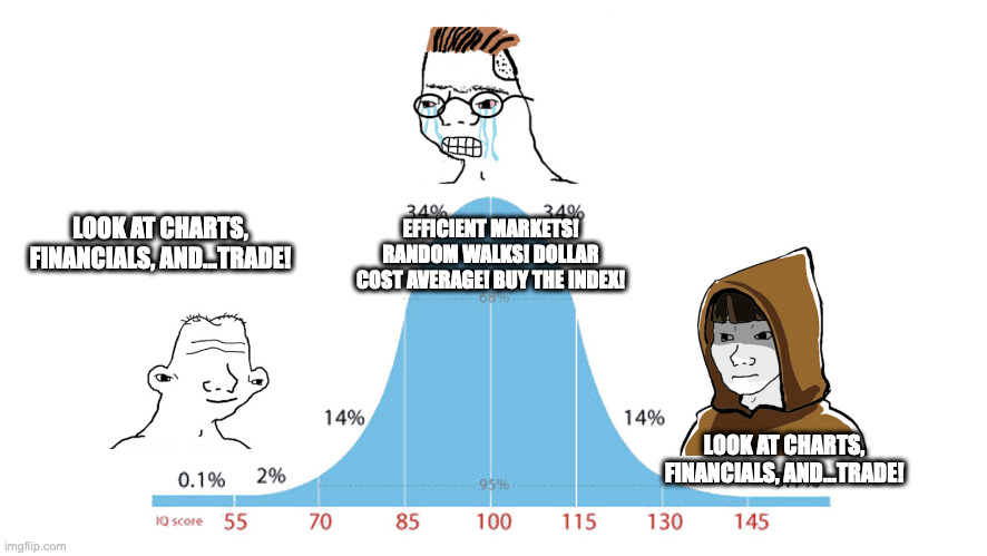
In retrospect, this sums up the way I think about markets:
I hope this essay helped you understand what it takes to build a fully productionized ML-powered stock picking engine from scratch. In terms of further reading, here are some references that helped me on my quest.
Books #
Note: These are Amazon Affiliate links; if you purchase any of these books using my links, the commissions I get will help pay for this blog. Thanks!
-
An Engine, Not A Camera, Donald MacKenzie - This book, more than any other, shaped the way I think about financial markets and finance as a subject of analysis. Though I talk about this in a related post, in short, it reinforced my assumptions of macroeconomics and finance as a narrative discipline first and an analytically-driven, quantitatively-rooted area of study later. In other words, human forces drive the models that underlie modern markets - as normative theories evolve on how markets should behave, market behavior reflects that change (e.g. the infamous volatility smile that appeared after the 1987 market crash, as participants learnt to treat downside and upside risks asymmetrically).
-
Lords of Finance: 1929, The Great Depression, and the Bankers who Broke the World, Liaquat Ahmad - On a closely-related theme, through the lens of the Great Depression, the author examines the biases and personal histories of the key decision makers running international finance in the 1920s, and the disproportionate roles that these biases played in prolonging the greatest economic malaise of the 20th century. Sometimes it pays to study the humans who are making the decisions that affect us, and mentally model the paths they are most likely to take, especially under pressure.
-
Active Equity Management, Xinfeng Zhou & Sameer Jain - This is a very useful compendium of information on the types of factors affecting equity returns. The authors cover a rich field of documented market anomalies and factors, with sources that include technical (price/volume), fundamental (financial statements), and macroeconomic signals. They also provide a great discussion on combining signals that is well worth the practitioner’s time.
-
Professional Automated Trading: Theory & Practice, Eugene Durenard - This is a great resource that walks readers through designing a trading engine. The code examples are in Common Lisp, but translating it to Python shouldn’t be a problem.
-
Advances in Financial Machine Learning, Marcos Lopez de Prado - MLDP (the author) is famous in the field for, among other things, having co-designed the VPIN metric that has been used to measure order flow toxicity triggered by HFT systems, and track and predict flash crashes. This is his first book that talks about a variety of considerations when performing ML on financial data. I have a few nitpicks with his approach (and the book’s general lack of structure), but overall I recommend reading this to reorient one’s thinking about ML in this domain.
-
How to Make Money in Stocks, William O’Neil - Ha! This is an oldie but goodie. If you ignore the corny title that begs for the book to be placed on the bottom shelf of the dingy self-help section in bookstores, this is one of the best introductions to thinking jointly (and conditionally) about both accounting-based as well as price/volume-based features that would be useful in a ML context. When designing trading systems, I am extremely agnostic as to how I derive unique features - if a feature is marginally useful, I put it on my list, regardless of whether it is perceived as technical analysis voodoo or rigorous financial statement analysis. This book covers plenty of real-world ideas to trigger one’s thinking about feature engineering. Note that the author wrote the first edition of this book in the early 1960s, and its age does show a bit, but the CANSLIM approach overall pays off really well during market regimes that reward growth stocks with strong revenue generation fundamentals (a regime that we last saw during the pandemic bull run).
Selected papers #
At this point, folks generally point to hoary old classic papers such as the one by Jegadeesh & Titman on the momentum anomaly. Though I won’t be able to perform an in-depth literature review at this stage (trade secrets, y’all :shrug:), I will instead do something that might be arguably better: provide references to some great foundational papers that helped me start thinking seriously and conduct research in this area. I promise you that following through the citation webs for these papers will help you create powerful automated stock pickers as well.
-
Gupta, Tarun and Kelly, Bryan T., Factor Momentum Everywhere (November 1, 2018). Yale ICF Working Paper No. 2018-23.
-
Mohanram, P.S. Separating Winners from Losers among Low Book-to-Market Stocks using Financial Statement Analysis. Rev Acc Stud 10, 133–170 (2005).
-
Leung, Edward and Lohre, Harald and Mischlich, David and Shea, Yifei and Stroh, Maximilian, The Promises and Pitfalls of Machine Learning for Predicting Stock Returns (March 27, 2020).
-
Brush, J. S. (1986). Eight relative strength models compared. The Journal of Portfolio Management, 13(1), 21–28.